
Explaining Backpropagation
Published:
This blog post aims to clear up backpropagation in neural networks and give a more intuitive understanding of how it works. Before starting, recall that the goal of a neural network is to learn the weights $W$ and biases $b$ that minimize some loss function $L$.
To demonstrate the backpropagation step, we’ll use an arbitrary 2 layer neural network designed for binary classification. The activation of the hidden layer is calculated via the ReLU function:
\[g(x) = max(0, x)\]and the activation of the output layer is calculated via the sigmoid function:
\[\sigma (x) = \frac{1}{1 + e^{-x}}\]We’ll use cross entropy as the loss function, where $y$ is the true label for a specific set of input features, and $A$ is the value the network calculated:
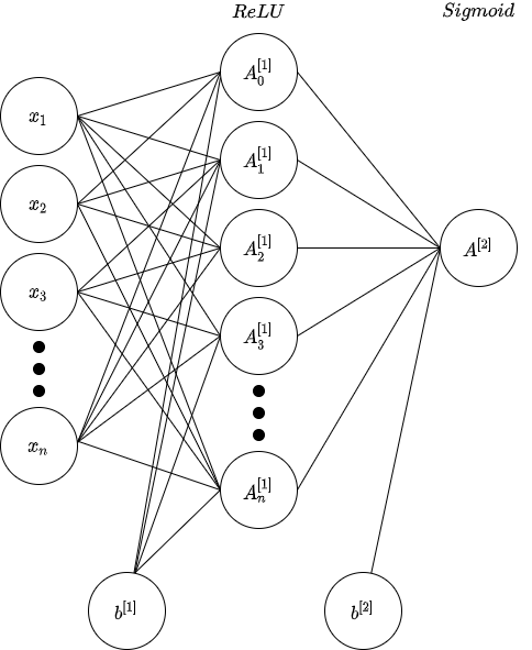
\[L = -y \ ln(A) - (1-y) \ ln(1-A)\]The architecture of the network is presented below. Note that the number of neurons isn’t relevant to the derivations, and additionally note that we’ll initialize the weights and biases for this network randomly.
We can write out all the necessary calculations for a successful forward pass as a computation graph:
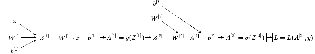
With this complete, we now know what the loss/error of the network is, but we need some way of minimizing $L$ by adjusting the biases and weights- in other words, achieving the goal of the network. As it turns out, we can use an algorithm called gradient descent to do this. For some function $f(x)$, the algorithm begins by selecting a random value for $x$ and then calculates the following equation (usually until some criteria is met, such as a loop count):
\[x^{current} = x^{previous} - \alpha \frac{dy}{dx}\]where $\alpha$ is a learning rate, that determines how large we want the update to be.
If you repeat this calculation long enough, $x^{current}$ will give you the point where the function $f(x)$ is at its lowest. When applied to neural networks, we can use this to find the weight and bias values that make the loss of the network ($L$) as low as possible. Since we essentially set $W$, $b$, and $\alpha$ ourselves, we only need to figure out the derivatives for $L$ with respect to weights and biases. Since we have 2 sets of weights and 2 sets of biases, we’ll end up with 4 gradient descent equations.
This is where the computation graph becomes useful. Using the computation graph, we can easily see the relationships between the various parts of the network: the loss depends on the activation of the second layer, the activation of the second layer depends on the net input of the second layer (i.e. $Z^{[2]}$), the net input depends on the weights and biases, and so on. By applying the chain rule to the computation graph, we can travel through the dependencies of the loss function and thereby express the loss function in terms of the weights and biases; exactly what we need for gradient descent. Note that these functions are multivariable, so we have to use partial derivatives.
Note: If you’re not totally comfortable with function relationships via the chain rule, this link gives a good explanation.
With that out of the way, we therefore need the following 4 equations to run gradient descent on all the weights and biases: $\frac{\partial L}{\partial W^{[2]}}, \frac{\partial L}{\partial b^{[2]}}, \frac{\partial L}{\partial W^{[1]}}, \frac{\partial L}{\partial b^{[1]}}$
For the second set of weights and biases we would have:
\[\frac{\partial L}{\partial W^{[2]}} = \frac{\partial L}{\partial A^{[2]}} \frac{\partial A^{[2]}}{\partial Z^{[2]}} \frac{\partial Z^{[2]}}{\partial W^{[2]}}\] \[\frac{\partial L}{\partial b^{[2]}} = \frac{\partial L}{\partial A^{[2]}} \frac{\partial A^{[2]}}{\partial Z^{[2]}} \frac{\partial Z^{[2]}}{\partial b^{[2]}}\]Before beginning the calculations, remember that you can treat the differentials here as fractions (even though they’re not), so $\frac{\partial L}{\partial A^{[2]}} \frac{\partial A^{[2]}}{\partial Z^{[2]}} = \frac{\partial L}{\partial Z^{[2]}} $ and vice versa. We now need to solve $\frac{\partial L}{\partial Z^{[2]}}$, we can work out the biases and weights from this result. Breaking it up into parts is the easiest way of doing it, we can start by working out $\frac{\partial L}{\partial A^{[2]}}$. Practically speaking, we calculate it as:
\[\frac{\partial L}{\partial A^{[2]}} = -\frac{y}{A^{[2]}} + \frac{1-y}{1-A^{[2]}}\]Next is $\frac{\partial A^{[2]}}{\partial Z^{[2]}}$:
\[\frac{\partial A^{[2]}}{\partial Z^{[2]}} = \sigma(Z^{[2]})(1-\sigma(Z^{[2]})) = A^{[2]}(1-A^{[2]})\]Calculating $\frac{\partial L}{\partial A^{[2]}} \frac{\partial A^{[2]}}{\partial Z^{[2]}}$ and simplifying gives the following result.
\[\frac{\partial L}{\partial Z^{[2]}} = A^{[2]} - y\]Finally we can substitute, then get the equations for the biases and weights:
\[\frac{\partial L}{\partial W^{[2]}} = (A^{[2]} - y) \cdot A^{[1]}\] \[\frac{\partial L}{\partial b^{[2]}} = A^{[2]} - y\]Now we need to calculate $\frac{\partial L}{\partial W^{[1]}}$ and $\frac{\partial L}{\partial b^{[1]}}$. The derivation of these equations is slightly longer because we now have to move back another layer:
\[\frac{\partial L}{\partial W^{[1]}} = \frac{\partial L}{\partial A^{[2]}} \frac{\partial A^{[2]}}{\partial Z^{[2]}} \frac{\partial Z^{[2]}}{\partial A^{[1]}} \frac{\partial A^{[1]}}{\partial Z^{[1]}} \frac{\partial Z^{[1]}}{\partial W^{[1]}}\] \[\frac{\partial L}{\partial b^{[1]}} = \frac{\partial L}{\partial A^{[2]}} \frac{\partial A^{[2]}}{\partial Z^{[2]}} \frac{\partial Z^{[2]}}{\partial A^{[1]}} \frac{\partial A^{[1]}}{\partial Z^{[1]}} \frac{\partial Z^{[1]}}{\partial b^{[1]}}\]Notice how we’re using the chain rule to “travel” backwards through activation functions and net inputs (i.e. $Z$) to find the update equations for the weights and biases in deeper layers. In my perspective, this is what the backward pass is about.
We’ve already calculated $\frac{\partial L}{\partial Z^{[2]}}$, we can simply calculate the rest of the variables then solve for the first layer’s weights and biases. Starting at $\frac{\partial Z^{[2]}}{\partial A^{[1]}}$:
\[\frac{\partial Z^{[2]}}{\partial A^{[1]}} = W^{[2]}\]The derivative of the ReLU function is a piecewise function:
\[g'(x) = \begin{cases} 1, \quad if \enspace x > 0 \\ 0, \quad otherwise \end{cases}\]therefore
\[\frac{\partial A^{[1]}}{\partial Z^{[1]}} = g'(Z^{[1]})\]Completing the rest and simplifying gives us:
\[\frac{\partial L}{\partial Z^{[1]}} = (A^{[2]} - y) \cdot W^{[2]} \cdot g'(Z^{[1]})\] \[\frac{\partial L}{\partial W^{[1]}} = \frac{\partial L}{\partial Z^{[1]}} \cdot A^{[0]}\] \[\frac{\partial L}{\partial b^{[1]}} = \frac{\partial L}{\partial Z^{[1]}}\]With all the equations solved, gradient descent can be implemented and the network can learn.
Although backpropagation is often seen as a challenging process to understand, when viewed as the process of calculating the weight update equations for gradient descent, it can make more sense. With any topic in Artificial Intelligence, learning the mathematical parts requires time, patience, and practice. As long as you maintain knowledge of calculus essentials, the learning process can go a little more smoothly.